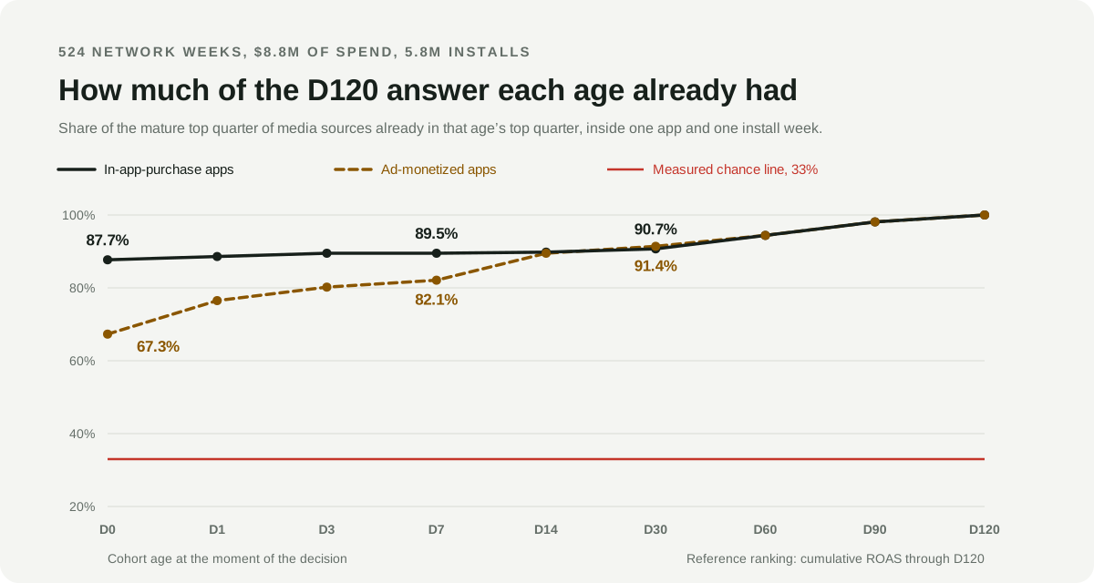
“Wait for D30” is standing advice in mobile UA, and we could not find a published measurement of what the wait returns. So we made one. We ranked media sources by cumulative ROAS at every cohort age from install day to D120, on 524 network weeks, $8.8M of spend and 5.8M installs, and counted how much of the mature ranking each age already had. On the in-app-purchase apps in the panel, the answer was 89.5% at D7 and 90.7% at D30. The 23 days of waiting bought 1.2 points. On the ad-monetized apps the same wait bought 9.3 points, from 82.1% to 91.4%.

There is no single decision age. There is a curve, it differs by app, and you can measure your own in an afternoon.

Same units, same scopes, read at nine cohort ages against the same D120 answer.

Two guides published two weeks apart give opposite advice

This is not settled advice we are re-litigating. It is a live disagreement between practitioners who both sound certain.

One current guide tells you to wait. Never compare channels on D7 alone, it says, because “a channel with a lower D7 ROAS can outperform a channel with a higher one once the full LTV curve plays out”, and judging every channel against the same D7 target “can lead a team to cut a campaign that would have paid off, and scale one that never will”. The illustration offered is a pair of channels, one at 20% ROAS on D7 that does not break even until D60, another that starts lower and reaches 100% by D30. Published August 17, 2026.

Another tells you the opposite, in the same month. “Wait until D30 and the budget is already spent. A D7 verdict separates campaigns to scale from campaigns to kill while the budget is still alive”, because “the first week’s revenue trajectory correlates strongly with the D30 and D90 curves”. Published August 10, 2026.

The older and more careful version of the sceptical case is Liftoff’s 2020 argument for retiring D7 ROAS, which shows that “Day 365 and Day 7 LTV are not proportional, nor should one expect them to be” and compares estimation methods on bootstrapped samples. That argument is about level accuracy: a D7 number multiplied by a fixed factor is a bad estimate of D365. It is correct and it is not the same question as whether the early table puts the right networks at the top.

Meanwhile the buying systems are not waiting either. Unity’s ROAS campaigns optimize on D7 and D28 windows for in-app purchase, and add a D0 window for ad revenue. A network willing to bid against install-day revenue is making a claim about how early the signal exists. All four sources verified August 24, 2026.

None of them publishes a measurement of the thing a UA lead actually needs: how much of next quarter’s answer is already in this week’s table.

The denominator settles on install day, which is what makes this measurable

Cumulative ROAS at day d is attributed revenue through day d divided by acquisition spend. The spend is fixed the moment the installs are bought. It does not move on day 8 or day 90.

So every reordering of a ROAS table between an early read and a mature read comes from one place: the revenue curve. If two networks trade places between D7 and D120, it is because their cumulative revenue grew at different rates, not because anything about the cost side was revised. That reduces a vague worry about early data to a single measurable question, and it is the question the two guides above disagree about without measuring.

It also means the interesting quantity is not accuracy. Nobody allocates budget by asking whether the D7 number equals the D120 number, because it obviously does not. They allocate by asking which network is ahead. That is an ordering, and orderings can be checked.

The test: rank the same units twice, at two ages

We took one comparison scope at a time, meaning one app and one install week, and ranked the media sources inside it by cumulative ROAS. Once using revenue through an early day. Once using revenue through D120. Then we counted how many of the top quarter of the mature ranking were already in the top quarter of the early one.

The early ages are D0, D1, D3, D7, D14, D30, D60 and D90. The reference is always the same D120 answer, so every age on the curve is scored against an identical target.

Four details keep the count honest.

Ties are broken at random and every ranking is drawn 25 times and averaged. Some units earn nothing on install day. A deterministic sort would put identical zeros in the same order in both readings and manufacture agreement out of nothing.

The chance line is measured, not assumed. With six units in a scope, a quarter is two units and a coin flip would score 33%, not 25%. Rather than trust that arithmetic, we permuted the reference ranking inside each scope 400 times, which reproduces the exact shape of these comparisons including the tie structure. The measured chance line came out at 33.5% for the in-app-purchase arm, 32.3% for the ad-monetized arm, and 25.6% for the finer geo cut described below.

Intervals come from 1,000 bootstrap resamples of whole scopes, not of individual units, so a single unusually stable app week cannot narrow the interval by itself.

Only cohorts observed all the way to day 120 are used. Rows in this warehouse refresh on a rolling schedule, so a cell last written at day 68 cannot contribute a D120 value. Requiring day 120 observation retains $9.05M of $12.22M of spend on the network arm and $2.16M of $5.25M on the geo arm. Both numerator and denominator come from the same retained rows, so the ratio stays internally consistent.

Units need $250 of spend and 100 installs to be ranked, scopes need at least five units, and retargeting rows are excluded throughout.

What the panel is

Arm	Grain	Scopes	Units	Spend	Installs
In-app-purchase apps	media source, install week	54	348	$6,808,088	3,843,049
Ad-monetized apps	media source, install week	27	176	$1,987,202	1,991,882
Ad-monetized apps, finer cut	media source and country, install month	9	519	$2,090,477	1,905,838

The first two arms are the headline panel: 524 units, $8,795,290 of spend, 5,834,931 installs, ten media sources inside each arm, install weeks from June 2024 to January 2026. The third arm re-cuts the same ad-monetized spend at a finer grain and is not added to the total.

One set of apps monetizes mainly through in-app purchases and the other mainly through advertising, which is what makes the contrast in the next two sections possible.

On the in-app-purchase apps, install day already knew

Cohort age	Share of the D120 top quarter already identified	95% interval	Spearman against D120
D0	87.7%	81.8 to 93.2	0.940
D1	88.6%	82.7 to 94.1	0.940
D3	89.5%	84.3 to 94.8	0.950
D7	89.5%	84.0 to 94.4	0.950
D14	89.8%	84.3 to 94.4	0.956
D30	90.7%	85.2 to 95.4	0.972
D60	94.4%	89.8 to 98.1	0.987
D90	98.1%	95.4 to 100	0.994

Against a measured chance line of 33.5%, the install-day ranking already held 87.7% of the mature answer. The entire journey from D0 to D30, a month of waiting, moved the count by three points, and the intervals overlap almost completely.

This is the case the sceptical advice says should not happen. It happened on $6.8M of spend across 54 app weeks.

On the ad-monetized apps, the first week did the work

Cohort age	Share of the D120 top quarter already identified	95% interval	Spearman against D120
D0	67.3%	55.6 to 77.8	0.751
D1	76.5%	67.3 to 85.2	0.826
D3	80.2%	71.6 to 88.9	0.865
D7	82.1%	72.8 to 90.7	0.907
D14	89.5%	82.1 to 96.3	0.927
D30	91.4%	84.0 to 98.1	0.930
D60	94.4%	88.9 to 100	0.975
D90	98.1%	94.4 to 100	0.992

Here the sceptics are closer to right, and only for the first few days. Install day carried 67.3% against a 32.3% chance line, which is well above chance and clearly not enough to act on. A week of data moved it to 82.1%. The next 23 days added 9.3 more points.

So the two app sets converge to the same place by D30 and get there on very different schedules. Read the two tables together and the practical lesson is not that D7 is fine or that D7 is dangerous. It is that the decision age is a property of the app, it varies by more than twenty points on install day between two app sets in the same panel, and neither of the guides quoted above can tell you which one you are.

More revenue in the books does not mean a more stable ranking

The obvious explanation for the gap would be that the in-app-purchase apps simply collect their revenue sooner. They do not.

Share of D120 revenue already booked	D0	D7	D30	D90
In-app-purchase apps	40%	50%	68%	92%
Ad-monetized apps	32%	73%	91%	99%

The ad-monetized apps are far ahead on revenue arrival at every age after install day. By D7 they have booked 73% of their D120 revenue against 50% for the purchase-led apps, and by D30 they are at 91%. Their ranking is nevertheless the less settled of the two at every age up to D14.

That is worth sitting with, because “how much revenue has arrived” is the intuition most teams reach for when they decide how long to wait. It is the wrong instrument. What determines when a ranking settles is not how much revenue has landed but whether the revenue that landed is a representative sample of what each unit will eventually produce. A handful of early in-app purchases apparently identify which network delivers payers. A large volume of install-day ad impressions apparently does not identify which network delivers durable sessions, at least not yet.

We can show that revenue share and ordering stability come apart. We cannot prove the mechanism from this panel, and the two app sets differ in monetization, network mix and calendar all at once. Treat the mechanism as a hypothesis and the divergence as the finding.

The mistake an early read makes is a false kill, not a false scale

An overall agreement rate hides which direction the errors run, and the two directions cost very different amounts.

Count the quarter slots directly rather than averaging rates. Across all three arms at D7, not one unit that the early reading placed in the top quarter finished in the mature bottom quarter: zero of 114 slots on the in-app-purchase arm, zero of 55 on the ad-monetized network arm, zero of 133 on the finer geo cut. The early read did not promote a single genuine loser.

The errors that did occur ran the other way, units the early reading placed in the bottom quarter that finished in the mature top quarter. At D7 that was zero of 114 slots on the in-app-purchase arm, one of 55 on the ad-monetized network arm, and two of 133 on the geo cut. On install day the ad-monetized network arm produced four false kills out of 55 slots, about one in fourteen, alongside two false scales.

That asymmetry is the operationally useful part. If the thing you fear is pouring budget into a network that early data flattered, this panel says that fear is close to unfounded from D7 onward. If the thing you fear is cutting a network that would have come good, that risk is real, it is small by D7, and it is several times larger on install day for an ad-monetized app.

It also suggests an obvious hedge that costs almost nothing. Act on the top of the early table and hold the bottom. Scaling decisions at D7 produced no false scales anywhere in this panel. Kill decisions are the ones worth a hold band, which is the same structure a D7 ROAS target set from your own mature cohorts uses when it puts a hold zone between the cut line and the scale line.

What the wait costs

The case for waiting is that the extra information is worth the delay. The case against it is that buying does not pause while you deliberate. That second half is measurable too, so we measured it rather than assuming a spend rate.

For every unit in the panel we took the D7 decision date, which is seven days after the install week closes, and added up what that same app and network actually spent on installs over the following 23 days, the interval between a D7 verdict and a D30 verdict.

App set	Median continuation per network decision	Total across decisions	Share into units both readings call bottom quarter
In-app-purchase apps	$30,570	$17,857,737 over 348 decisions	40.2%
Ad-monetized apps	$38,211	$8,870,282 over 176 decisions	16.8%

The median deferred decision cost about $30,570 on the purchase-led apps and $38,211 on the ad-monetized ones. In both sets the continuation spend runs to several times the spend of the week being judged: a median of 2.72 times on the first set and 5.12 times on the second, because a weekly cohort is judged against 23 days of subsequent buying.

Set that against what the wait returned. On the in-app-purchase apps, 1.2 points of additional agreement, an amount smaller than the width of the confidence interval, in exchange for a median $30,570 per network decision. On the ad-monetized apps, 9.3 points for a median $38,211. The first trade is bad, the second is arguable, and neither is the trade the universal rule assumes you are making.

Two honest qualifications. Spending during the wait is not spending wasted, because those installs are still bought and still monetize. The number is the exposure a deferred verdict carries, not a loss. And 40.2% of the deferred spend on the purchase-led apps flowed into units that both the D7 reading and the mature reading placed in the bottom quarter, which is the portion where the delay bought nothing that either reading would have used.

What survives when you take away the easy networks

The strongest objection to the in-app-purchase result is that its scopes contain Apple Search Ads, a structurally different source that any reading gets right, and that the apparent stability is one large persistent gap rather than a ranking. That objection is right about the mechanism and wrong about the size.

Cut	Scopes	Units	Spend	D0	D7	D30	D60
In-app-purchase, all networks	54	348	$6,808,088	87.7%	89.5%	90.7%	94.4%
In-app-purchase, Apple removed	35	218	$3,559,128	81.4%	87.1%	88.6%	90.0%
In-app-purchase, Apple and Google removed	23	135	$1,747,303	78.3%	82.6%	87.0%	89.1%
In-app-purchase, scopes with 7 or more units	23	181	$3,034,415	81.9%	84.1%	89.1%	93.5%
Ad-monetized, all networks	27	176	$1,987,202	67.3%	82.1%	91.4%	94.4%
Ad-monetized, self-attributing networks removed	12	70	$700,273	66.7%	70.8%	79.2%	95.8%

Removing Apple costs the install-day figure 6.3 points and the D7 figure 2.4. Removing Apple and Google costs 9.4 and 6.9. Requiring larger scopes, which makes the ranking task harder, costs 5.8 and 5.4. The chance line was recomputed for every cut and ranges from 28.6% to 34.6%, so every row above sits far clear of it, and in every purchase-led cut the D7 to D30 step stays small.

The ad-monetized arm is more fragile. Removing the self-attributing networks leaves 12 scopes and $700,273, and on that thin cut D7 falls to 70.8% and the D7 to D30 step widens to 8.4 points. Read that row as a caution rather than a result.

Two more checks did not change the shape. Raising the spend floor from $250 to $1,000 per unit moved the in-app-purchase curve to 89.1% at D0, 90.1% at D7 and 91.3% at D30, and the ad-monetized curve to 61.9%, 81.0% and 88.1%. Moving the reference horizon from D120 to D90 reproduced both curves.

The finer geo cut is the one place the picture gets meaningfully worse. Ranking media source and country pairs inside an install month, which puts a median of 55 units in a scope instead of six, the D7 figure falls to 80.6% and D30 to 86.3% against a 25.6% chance line. Splitting a table finer makes the ordering harder to reproduce, which is the same relationship the creative test reliability study found when it pushed a revenue ranking down to asset grain. Nothing here says a campaign-level or asset-level table settles as early as a network-level one, and the direction of the geo result says it probably does not.

Run this on your own account before you trust any of it

The method is an overlap count. It needs one query and no model.

Pick a mature horizon your finance function actually uses, and only use install cohorts old enough to have reached it. If your revenue data thins out or changes resolution past a certain day, put the horizon before that point rather than reaching past it.
Fix one comparison scope. One app, one install week or month, one attribution definition, one revenue basis. The scope discipline is the same one the D7 ROAS target guide sets out, and it matters here for the same reason: pooling incomparable cohorts to raise the row count changes the question.
Rank your units by cumulative ROAS at each candidate decision age and again at the mature horizon. Count how many of the mature top quarter appear in each early top quarter. Break ties at random and average over a few dozen draws.
Permute the mature ranking inside each scope a few hundred times to get your own chance line. Do not assume 25%. With six units it is 33%.
Read the curve, not a single number. The decision age you want is the earliest age where the curve has flattened. On the purchase-led apps here that is install day for the full panel and closer to D7 once the largest structural gap between sources is removed. On the ad-monetized apps it is between D7 and D14.
Split the errors. Compute false scale and false kill separately. They justify different rules, and in this panel only one of them was worth designing around.
Price the wait. Add up what your accounts actually spent between two candidate decision dates. That number belongs in the decision, and it is usually larger than people expect.

The floors used here, $250 of spend and 100 installs per unit and five units per scope, were chosen to keep the panel wide. They are not correct for anyone else. Your own curve, computed on your own volumes, is the only decision age with evidence behind it.

What this does not establish

This is a narrow panel, not a market sample. It covers a small number of apps across two monetization profiles, one set monetizing mainly through purchases and the other mainly through advertising. An app with a slow-blooming revenue curve, a subscription product whose trials convert in week two, or a portfolio buying across forty networks instead of ten could produce a different curve. What we expect to transfer is the shape of the exercise, not these percentages.

The units are media sources, and a country cut for two of the apps. Not campaigns, not ad sets, not creatives. The one time we cut finer, agreement fell. Anyone applying this at campaign or asset grain should measure it there rather than importing these numbers, and should expect a later decision age.

The early figures are read from today’s restated table, not from a snapshot taken on the day. The D7 column here is what D7 looks like after every correction has landed. A team reading their dashboard on the actual day would have seen a noisier number, and the gap is wider for ad revenue, which restates on a schedule of its own. That makes every figure on this page an upper bound on what an early read could have told you at the time, which cuts against our own conclusion and is the reason it is stated plainly. The same distinction between a decision-time snapshot and a corrected history is what the forecast backtest audit exists to enforce.

A surviving ordering is not accuracy in level, and it is not causality. This page measures which unit is ahead. It says nothing about what any unit will earn, and nothing about whether moving budget toward the leader would produce more revenue, because the delivery was allocated by systems whose reasoning is not in this data. Ordering stability is a floor a metric clears before it is worth acting on, not a substitute for a forecast.

ROAS here is attributed revenue over aligned spend, with no store-fee netting and one fixed attribution definition per app. Change the attribution basis or the revenue basis and the ranking can change with it, which is why step two above insists on freezing them. The definitions and reconciliation rules are published in our methodology.

Where Lemon fits

Nothing above requires Lemon. It is an overlap count on cohort data you already own, and the conclusion is a change to when you read the table, not to what you buy.

What Lemon does is remove the reason most teams never run it. The measurement needs cumulative revenue by day since install, joined to aligned spend, at a stable grain, across every network, held far enough back in history that the cohorts have matured. That join is the work. Cohort Prediction maintains it as a product surface, with actual and predicted values kept visually distinct so nobody accidentally backtests a forecast against itself, and the reporting API exposes the same panel to a query or an agent when you would rather compute your own curve than read ours.

For the wider discipline, start with cohort revenue forecasting for mobile apps. Once you know your decision age, set the threshold you apply at that age from your own mature cohorts rather than from a benchmark.

What Waiting From D7 to D30 Actually Buys